Take Home Exercise 1

Author

You Ting Quek

Published

April 15, 2024

Modified

Invalid Date

Assignment Context

There are two major residential property market in Singapore, namely public and private housing. Public housing aims to meet the basic need of the general public with monthly household income less than or equal to S$14,000. For families with monthly household income more than S$14,000, they need to turn to the private residential market.

The Task

Assuming the role of a graphical editor of a median company, you are requested to prepare minimum two and maximum three data visualisation to reveal the private residential market and sub-markets of Singapore for the 1st quarter of 2024

Data Source

To accomplish the task, transaction data of REALIS (2023-2024) will be used.

Research

Prior to kickstarting the project, the author must first do some preliminary research on the local property market in Singapore as well as the factors that may contribute to it’s pricing.

The data provided by Realis are at it’s crux Transaction data, the author upon further research understands there are crucial determinant factors such as :

1.) Regions https://www.propertyguru.com.sg/property-guides/ccr-ocr-rcr-region-singapore-ura-map-21045

2.) And age of the property https://www.businesstimes.com.sg/property/price-gap-between-resale-condos-ccr-and-rcr-smallest-22-years-orangetee-tie

Setting up the environment

Installing required packages

pacman::p_load(tidyverse, ggplot2, dplyr, shiny, bslib)

Preparing the data

Raw Data Import

Given that there are 5 sets of Transaction CSV files, we will need to open each and every single one of them using read_csv function before merging them together again into 1 data frame.

Code
Output

# Define the paths to the individual CSV files
file1 <- "data/ResidentialTransaction20240308160536.csv"
file2 <- "data/ResidentialTransaction20240308160736.csv"
file3 <- "data/ResidentialTransaction20240308161009.csv"
file4 <- "data/ResidentialTransaction20240308161109.csv"
file5 <- "data/ResidentialTransaction20240414220633.csv"

# Reading the individual CSV files
data1 <- read_csv(file1)
data2 <- read_csv(file2)
data3 <- read_csv(file3)
data4 <- read_csv(file4)
data5 <- read_csv(file5)

# Combining the data frames into one
combined_transaction <- bind_rows(data1, data2, data3, data4, data5)

# Viewing the data structure given
col_names <- names(combined_transaction)
col_names

 [1] "Project Name"                "Transacted Price ($)"       
 [3] "Area (SQFT)"                 "Unit Price ($ PSF)"         
 [5] "Sale Date"                   "Address"                    
 [7] "Type of Sale"                "Type of Area"               
 [9] "Area (SQM)"                  "Unit Price ($ PSM)"         
[11] "Nett Price($)"               "Property Type"              
[13] "Number of Units"             "Tenure"                     
[15] "Completion Date"             "Purchaser Address Indicator"
[17] "Postal Code"                 "Postal District"            
[19] "Postal Sector"               "Planning Region"            
[21] "Planning Area"

Using glimpse to ensure our tibble dataframe is correct

glimpse (combined_transaction)

Rows: 26,806
Columns: 21
$ `Project Name`                <chr> "THE REEF AT KING'S DOCK", "URBAN TREASU…
$ `Transacted Price ($)`        <dbl> 2317000, 1823500, 1421112, 1258112, 1280…
$ `Area (SQFT)`                 <dbl> 882.65, 882.65, 1076.40, 1033.34, 871.88…
$ `Unit Price ($ PSF)`          <dbl> 2625, 2066, 1320, 1218, 1468, 1767, 1095…
$ `Sale Date`                   <chr> "01 Jan 2023", "02 Jan 2023", "02 Jan 20…
$ Address                       <chr> "12 HARBOURFRONT AVENUE #05-32", "205 JA…
$ `Type of Sale`                <chr> "New Sale", "New Sale", "New Sale", "New…
$ `Type of Area`                <chr> "Strata", "Strata", "Strata", "Strata", …
$ `Area (SQM)`                  <dbl> 82.0, 82.0, 100.0, 96.0, 81.0, 308.7, 42…
$ `Unit Price ($ PSM)`          <dbl> 28256, 22238, 14211, 13105, 15802, 19015…
$ `Nett Price($)`               <chr> "-", "-", "-", "-", "-", "-", "-", "-", …
$ `Property Type`               <chr> "Condominium", "Condominium", "Executive…
$ `Number of Units`             <dbl> 1, 1, 1, 1, 1, 1, 1, 1, 1, 1, 1, 1, 1, 1…
$ Tenure                        <chr> "99 yrs from 12/01/2021", "Freehold", "9…
$ `Completion Date`             <chr> "Uncompleted", "Uncompleted", "Uncomplet…
$ `Purchaser Address Indicator` <chr> "HDB", "Private", "HDB", "HDB", "HDB", "…
$ `Postal Code`                 <chr> "097996", "419535", "269343", "269294", …
$ `Postal District`             <chr> "04", "14", "27", "27", "28", "19", "10"…
$ `Postal Sector`               <chr> "09", "41", "26", "26", "79", "54", "27"…
$ `Planning Region`             <chr> "Central Region", "East Region", "North …
$ `Planning Area`               <chr> "Bukit Merah", "Bedok", "Yishun", "Yishu…

duplicates <- combined_transaction %>% 
  filter(duplicated(.))
glimpse(duplicates)

Rows: 0
Columns: 21
$ `Project Name`                <chr> 
$ `Transacted Price ($)`        <dbl> 
$ `Area (SQFT)`                 <dbl> 
$ `Unit Price ($ PSF)`          <dbl> 
$ `Sale Date`                   <chr> 
$ Address                       <chr> 
$ `Type of Sale`                <chr> 
$ `Type of Area`                <chr> 
$ `Area (SQM)`                  <dbl> 
$ `Unit Price ($ PSM)`          <dbl> 
$ `Nett Price($)`               <chr> 
$ `Property Type`               <chr> 
$ `Number of Units`             <dbl> 
$ Tenure                        <chr> 
$ `Completion Date`             <chr> 
$ `Purchaser Address Indicator` <chr> 
$ `Postal Code`                 <chr> 
$ `Postal District`             <chr> 
$ `Postal Sector`               <chr> 
$ `Planning Region`             <chr> 
$ `Planning Area`               <chr>

Data Analysis

Using glimpse() as a dipstick to run through our duplicate() checks, we concluded that the data is very sanitised with 0 duplicated transactions.

However we noted that there is an unsuitable data type for the field ‘Sale Date’ which will result in difficulty for us not being able to do filtering later on.

Filtering Q1 2024 data for Private properties

combined_transaction$`Sale Date` <- dmy(combined_transaction$`Sale Date`)

# Check the structure to ensure 'Sale Date' is now a Date object
str(combined_transaction)

Q1_2024_Private <- combined_transaction %>%
  filter(`Sale Date` >= as.Date("2023-01-01") & 
         `Sale Date` <= as.Date("2024-03-31"))

head(Q1_2024_Private)

combined_transaction$`Sale Date` <- dmy(combined_transaction$`Sale Date`)

# Check the structure to ensure 'Sale Date' is now a Date object
str(combined_transaction)

spc_tbl_ [26,806 × 21] (S3: spec_tbl_df/tbl_df/tbl/data.frame)
 $ Project Name               : chr [1:26806] "THE REEF AT KING'S DOCK" "URBAN TREASURES" "NORTH GAIA" "NORTH GAIA" ...
 $ Transacted Price ($)       : num [1:26806] 2317000 1823500 1421112 1258112 1280000 ...
 $ Area (SQFT)                : num [1:26806] 883 883 1076 1033 872 ...
 $ Unit Price ($ PSF)         : num [1:26806] 2625 2066 1320 1218 1468 ...
 $ Sale Date                  : Date[1:26806], format: "2023-01-01" "2023-01-02" ...
 $ Address                    : chr [1:26806] "12 HARBOURFRONT AVENUE #05-32" "205 JALAN EUNOS #08-02" "29 YISHUN CLOSE #08-10" "45 YISHUN CLOSE #07-42" ...
 $ Type of Sale               : chr [1:26806] "New Sale" "New Sale" "New Sale" "New Sale" ...
 $ Type of Area               : chr [1:26806] "Strata" "Strata" "Strata" "Strata" ...
 $ Area (SQM)                 : num [1:26806] 82 82 100 96 81 ...
 $ Unit Price ($ PSM)         : num [1:26806] 28256 22238 14211 13105 15802 ...
 $ Nett Price($)              : chr [1:26806] "-" "-" "-" "-" ...
 $ Property Type              : chr [1:26806] "Condominium" "Condominium" "Executive Condominium" "Executive Condominium" ...
 $ Number of Units            : num [1:26806] 1 1 1 1 1 1 1 1 1 1 ...
 $ Tenure                     : chr [1:26806] "99 yrs from 12/01/2021" "Freehold" "99 yrs from 15/02/2021" "99 yrs from 15/02/2021" ...
 $ Completion Date            : chr [1:26806] "Uncompleted" "Uncompleted" "Uncompleted" "Uncompleted" ...
 $ Purchaser Address Indicator: chr [1:26806] "HDB" "Private" "HDB" "HDB" ...
 $ Postal Code                : chr [1:26806] "097996" "419535" "269343" "269294" ...
 $ Postal District            : chr [1:26806] "04" "14" "27" "27" ...
 $ Postal Sector              : chr [1:26806] "09" "41" "26" "26" ...
 $ Planning Region            : chr [1:26806] "Central Region" "East Region" "North Region" "North Region" ...
 $ Planning Area              : chr [1:26806] "Bukit Merah" "Bedok" "Yishun" "Yishun" ...
 - attr(*, "spec")=
  .. cols(
  ..   `Project Name` = col_character(),
  ..   `Transacted Price ($)` = col_number(),
  ..   `Area (SQFT)` = col_number(),
  ..   `Unit Price ($ PSF)` = col_number(),
  ..   `Sale Date` = col_character(),
  ..   Address = col_character(),
  ..   `Type of Sale` = col_character(),
  ..   `Type of Area` = col_character(),
  ..   `Area (SQM)` = col_number(),
  ..   `Unit Price ($ PSM)` = col_number(),
  ..   `Nett Price($)` = col_character(),
  ..   `Property Type` = col_character(),
  ..   `Number of Units` = col_double(),
  ..   Tenure = col_character(),
  ..   `Completion Date` = col_character(),
  ..   `Purchaser Address Indicator` = col_character(),
  ..   `Postal Code` = col_character(),
  ..   `Postal District` = col_character(),
  ..   `Postal Sector` = col_character(),
  ..   `Planning Region` = col_character(),
  ..   `Planning Area` = col_character()
  .. )
 - attr(*, "problems")=<externalptr>

Q1_2024_Private <- combined_transaction %>%
  filter(`Sale Date` >= as.Date("2023-01-01") & 
         `Sale Date` <= as.Date("2024-03-31"))

head(Q1_2024_Private)

# A tibble: 6 × 21
  `Project Name`       `Transacted Price ($)` `Area (SQFT)` `Unit Price ($ PSF)`
  <chr>                                 <dbl>         <dbl>                <dbl>
1 THE REEF AT KING'S …                2317000          883.                 2625
2 URBAN TREASURES                     1823500          883.                 2066
3 NORTH GAIA                          1421112         1076.                 1320
4 NORTH GAIA                          1258112         1033.                 1218
5 PARC BOTANNIA                       1280000          872.                 1468
6 NANYANG PARK                        5870000         3323.                 1767
# ℹ 17 more variables: `Sale Date` <date>, Address <chr>, `Type of Sale` <chr>,
#   `Type of Area` <chr>, `Area (SQM)` <dbl>, `Unit Price ($ PSM)` <dbl>,
#   `Nett Price($)` <chr>, `Property Type` <chr>, `Number of Units` <dbl>,
#   Tenure <chr>, `Completion Date` <chr>, `Purchaser Address Indicator` <chr>,
#   `Postal Code` <chr>, `Postal District` <chr>, `Postal Sector` <chr>,
#   `Planning Region` <chr>, `Planning Area` <chr>

Data Visualisation

Transaction Type Distribution across Planning Regions on Different Private Residential Types in 1st Quarter 2024

From our initial peek into the available data attributes, there are a few key attributes which we believe is useful in revealing interesting observable trends such as Planning Region, PSF price and Property types.

To test this hypothesis, we will use a FacetGrid to show the significance each metric has on the total transactions.

ggplot(data=Q1_2024_Private, 
       aes(x = `Unit Price ($ PSF)`, 
           fill = `Type of Sale`)) +
  geom_histogram(position = "dodge", binwidth = 100) +  # Adjust binwidth as needed
  facet_grid(`Planning Region` ~ `Property Type`) +
  labs(x = "PSF Price", y = "Count", title = "Distribution of PSF Prices by Property Type, Region, and Transaction Type") +
  scale_fill_brewer(palette = "Set1") +  # Use a color palette that is distinct
  theme_minimal() +
  theme(legend.position = "bottom")  # Adjust legend position as needed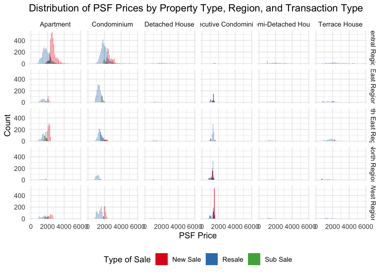

ggplot(data=Q1_2024_Private, 
       aes(x = `Planning Region`, 
           fill = `Property Type`)) +
  geom_bar(color = "grey30") +
  labs(x = "Region", y = "Transactions", title = "Sale of different property types in different Regions") +
  theme_minimal()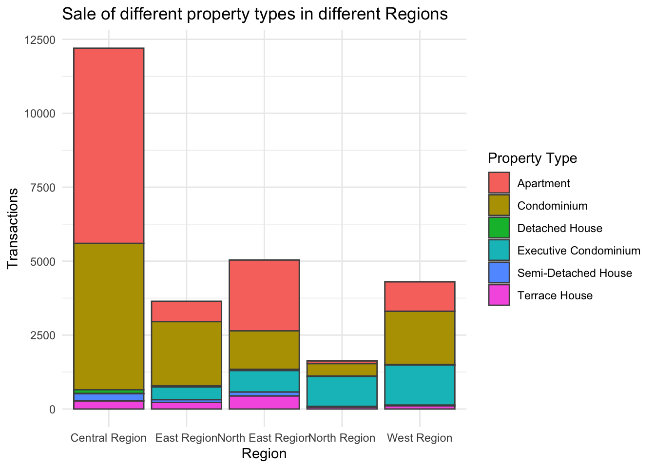

Observation from the Drilldown chart

From the FacetGrid transaction volumes of Property Types segregated by the different regions, we observed that majority of the transactions happening in 2024 involves either Apartments or Condominiums in the Central Region.

Shifting gears into the types of sale, we can also observe that New Sale is very popular for Apartments in Central Region as well as Executive Condominiums in the West Region. This sentiment is also backed by Straits Times

Given that the graph has highlighted Region and Apartment Type has a high correlation in contributing to buyer’s interest, we have use a histogram to illustrate it in the drilldown chart.

Average Transaction Price by Sale Type and Region

Using Geospatial mapping later, we notice can now see clearly from a macro POV that the price distribution by PSF in Singapore.

However, our literature research also shows that there are experts who claims that prices of properties are also affected by their age and sale type.

library(ggthemes)

q1_psf <- Q1_2024_Private %>%
  group_by(`Type of Sale` , `Planning Region`) %>%
  summarize(`Average PSF` = mean(`Unit Price ($ PSF)`), .groups = "drop")
q1_psf

# A tibble: 15 × 3
   `Type of Sale` `Planning Region` `Average PSF`
   <chr>          <chr>                     <dbl>
 1 New Sale       Central Region            2682.
 2 New Sale       East Region               1793.
 3 New Sale       North East Region         2161.
 4 New Sale       North Region              1319.
 5 New Sale       West Region               1911.
 6 Resale         Central Region            1895.
 7 Resale         East Region               1369.
 8 Resale         North East Region         1440.
 9 Resale         North Region              1213.
10 Resale         West Region               1376.
11 Sub Sale       Central Region            2154.
12 Sub Sale       East Region               1659.
13 Sub Sale       North East Region         1729.
14 Sub Sale       North Region              1485 
15 Sub Sale       West Region               1995.

# Calculate overall mean of 'Average PSF'
overall_mean <- mean(q1_psf$`Average PSF`)

ggplot(q1_psf, aes(x = `Planning Region`, y = `Average PSF`, fill = `Type of Sale`)) +
  geom_bar(stat = "identity", position = position_dodge()) +
  geom_hline(yintercept = overall_mean, linetype = "dashed", color = "black") +
  theme_minimal() +
  labs(title = "Average PSF by Region and Type of Sale",
       x = "Planning Region",
       y = "Average PSF",
       fill = "Type of Sale") +
  scale_fill_manual(values = c("New Sale" = "blue", "Resale" = "red", "Sub Sale" = "orange")) +   annotate("text", x = Inf, y = overall_mean, label = paste("Average PSF:", round(overall_mean, 2)), 
           vjust = -0.5, hjust = 1.1, color = "black", size = 3.5)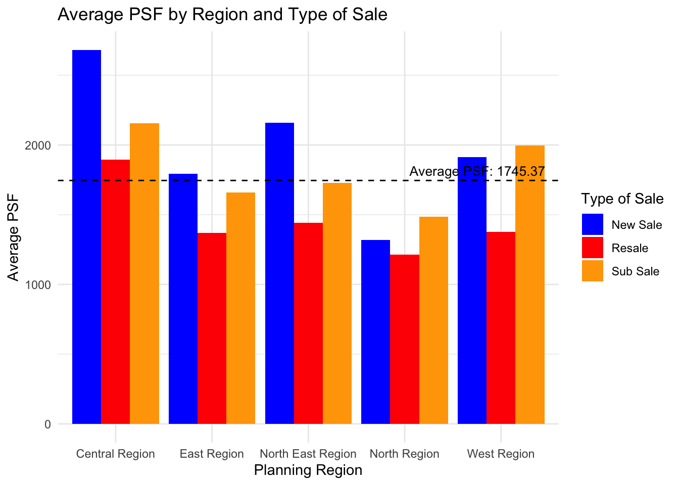

Observation of PSF prices for all transactions

Observing the bar chart, we can note that the Central Region exhibits the highest Average PSF for new sales, which is significantly above the overall average. In contrast, the North Region presents the lowest Average PSF figures for both new sales and resales.

Lastly, the chart also shows a clear trend where new sales consistently have higher Average PSF values compared to resales across all regions. The additional category of ‘Sub Sale’—present only for the East Region—falls below the overall mean. The overall mean PSF, marked by the dashed line, lies just below the Average PSF for resales in the Central Region, suggesting a higher concentration of sales with above-average prices in that region.

[Additional Bonus] Average Transaction Price by Region

To visualise the variation in average property prices across different regions in Singapore, we will use a choropleth map and shade each region according to its average property price which makes pricing differences immediately obvious.

To create the map, we will need the sub-zone boundary of URA Master Plan 2019 dataset as well as our own Q1_2024_Private dataset which we created earlier on.

The tools required are :

pacman::p_load(tmap,sf, httr, dplyr, future, furrr)

Components	Description
tmap	The syntax for creating plots is similar to that of `ggplot2`, but tailored to maps
sf	Support for simple features, a standardized way to encode spatial vector data
httr2	Create and submit HTTP requests and work with the HTTP responses
future	For sequential and parallel processing of R expression. This will be useful for expediting processing time later on.

Step 1

The first step is to utilise Singapore’s OneMap service to map each postal code to their corresponding Longtidue and Latitude.

cache <- new.env()
plan(multisession)

fetch_geocode_data <- function(postcode)
  # Check cache first
  if (exists(postcode, envir = cache)) {
    return(get(postcode, envir = cache))
  }
  
  # API parameters
  url <- "https://www.onemap.gov.sg/api/common/elastic/search"
  query_params <- list(searchVal = postcode, returnGeom = 'Y', getAddrDetails = 'Y', pageNum = '1')

  # API call with error handling
  response <- tryCatch({
    GET(url, query = query_params)
  }, error = function(e) {
    message("Error fetching data for postcode ", postcode, ": ", e$message)
    return(NULL)
  })

  # Check if the API call was successful
  if (is.null(response) || http_error(response)) {
    return(data.frame(postcode = postcode, lat = NA, lon = NA))
  }

  # Parse response
  content_data <- content(response, type = "application/json")

  # Store in cache and return results
  if (content_data$found > 0) {
    lat <- content_data$results[[1]]$LATITUDE
    lon <- content_data$results[[1]]$LONGITUDE
    result <- data.frame(postcode = postcode, lat = lat, lon = lon)
  } else {
    result <- data.frame(postcode = postcode, lat = NA, lon = NA)
  }

  assign(postcode, result, envir = cache)
  return(result)

##Output

cache <- new.env()
plan(multisession)

fetch_geocode_data <- function(postcode) {
  # Check cache first
  if (exists(postcode, envir = cache)) {
    return(get(postcode, envir = cache))
  }
  
  # API parameters
  url <- "https://www.onemap.gov.sg/api/common/elastic/search"
  query_params <- list(searchVal = postcode, returnGeom = 'Y', getAddrDetails = 'Y', pageNum = '1')

  # API call with error handling
  response <- tryCatch({
    GET(url, query = query_params)
  }, error = function(e) {
    message("Error fetching data for postcode ", postcode, ": ", e$message)
    return(NULL)
  })

  # Check if the API call was successful
  if (is.null(response) || http_error(response)) {
    return(data.frame(postcode = postcode, lat = NA, lon = NA))
  }

  # Parse response
  content_data <- content(response, type = "application/json")

  # Store in cache and return results
  if (content_data$found > 0) {
    lat <- content_data$results[[1]]$LATITUDE
    lon <- content_data$results[[1]]$LONGITUDE
    result <- data.frame(postcode = postcode, lat = lat, lon = lon)
  } else {
    result <- data.frame(postcode = postcode, lat = NA, lon = NA)
  }

  assign(postcode, result, envir = cache)
  return(result)
}

Step 2

We will now match Transaction (Q1_2024_Private) Tibble Dataframe’s unique postal code to our list of postal code extracted from OneMap.

# Search 'Q1_2024_Private' dataframe for 'Postal Code' column
data_pc <- unique(Q1_2024_Private$`Postal Code`)

# Use futures for asynchronous processing
results <- future_map(data_pc, fetch_geocode_data)
combined_results <- bind_rows(results)

# Combine results and filter out unsuccessful ones
successful_results <- combined_results %>%
  filter(!is.na(lat) & !is.na(lon))

# Write results to a CSV file
write.csv(successful_results, file = "data/PostalCodeList.csv", row.names = FALSE)

Q1_2024_Private_with_Coordinates <- Q1_2024_Private %>%
  left_join(successful_results, by = c("Postal Code" = "postcode"))

Step 3 Importing Geospatial Data

Load Map into MPSZ

# Instantiate the map from MPSZ 2019
mpsz <- st_read(dsn = "data/",
                layer = "MPSZ-2019") %>%
  st_transform(crs = 3414)

Reading layer `MPSZ-2019' from data source 
  `/Users/youting/ytquek/ISSS608-VAA/take_home_ex/data' using driver `ESRI Shapefile'
Simple feature collection with 332 features and 6 fields
Geometry type: MULTIPOLYGON
Dimension:     XY
Bounding box:  xmin: 103.6057 ymin: 1.158699 xmax: 104.0885 ymax: 1.470775
Geodetic CRS:  WGS 84

# Remove rows where latitude or longitude is NA
Q1_2024_Private_with_Coordinates <- Q1_2024_Private_with_Coordinates %>%
  filter(!is.na(lat) & !is.na(lon))

q1_2024_sf <- st_as_sf(Q1_2024_Private_with_Coordinates ,
                       coords = c("lon", "lat"),
                       crs =4326) %>%
  st_transform(crs = 3414)

Step 4 - Extracting study data (Average Transacted Price)

We will filter out the column data - Transacted Price, PSF & Planning Area which is required for a drill-down analysis on consumer pattern.

q1_avg_txn <- Q1_2024_Private_with_Coordinates %>%
    group_by(`Planning Area`) %>%
    summarise(Avg_Transacted_Price = mean(`Transacted Price ($)`, na.rm = TRUE))
q1_avg_txn <- q1_avg_txn %>%
    mutate(`Planning Area` = toupper(`Planning Area`))
q1_avg_txn <- st_drop_geometry(q1_avg_txn)

q1_avg_psf <- Q1_2024_Private_with_Coordinates %>%
    group_by(`Planning Area`) %>%
    summarise(Avg_Transacted_PSF = mean(`Unit Price ($ PSF)`, na.rm = TRUE))
q1_avg_psf <- q1_avg_psf %>%
    mutate(`Planning Area` = toupper(`Planning Area`))
q1_avg_psf <- st_drop_geometry(q1_avg_psf)

Step 5 - Geospatial Data Wrangling

Average Transacted Price ( Planning Region )
Average PSF ( Planning Region )

mpsz_avg_txn_px <- mpsz %>%
    left_join(
        q1_avg_txn,
        by = c("PLN_AREA_N" = "Planning Area")
    ) %>% drop_na()

tmap_mode("view")

map2 <- tm_shape(mpsz_avg_txn_px) +
    tm_polygons(col = "Avg_Transacted_Price", 
                palette = "YlOrRd",
                alpha = 0.3,
                style = "quantile",
                n = 7) +
    tmap_options(check.and.fix = TRUE) +
  tm_view(set.zoom.limits = c(11,14))

map2

mpsz_avg_psf <- mpsz %>%
    left_join(
        q1_avg_psf,
        by = c("PLN_AREA_N" = "Planning Area")
    ) %>% drop_na()

tmap_mode("view")

map3 <- tm_shape(mpsz_avg_psf) +
    tm_polygons(col = "Avg_Transacted_PSF",
                palette = "YlOrRd", 
                alpha = 0.3,
                style = "quantile",
                n = 7) +
    tmap_options(check.and.fix = TRUE) +
  tm_view(set.zoom.limits = c(11,14))

map3