In class exercise 4

pacman::p_load(tidyverse, ggstatsplot)

exam <- read_csv("data/Exam_data.csv")

set.seed(1234)

p <- gghistostats(
  data = exam,
  x = ENGLISH,
  type = "robust",
  test.value = 60,
  bin.args = list(color = "black",
                  fill = "grey 50",
                  alpha = 0.7),
  normal.curve = FALSE,
  normal.curve.args = list(linewidth = 2),
  xlab = "English scores"
)

##get the numbers
extract_stats(p)

$subtitle_data
# A tibble: 1 × 10
  statistic p.value n.obs method                                 effectsize  
      <dbl>   <dbl> <int> <chr>                                  <chr>       
1      11.1       0   322 Bootstrap-t method for one-sample test Trimmed mean
  estimate conf.level conf.low conf.high expression
     <dbl>      <dbl>    <dbl>     <dbl> <list>    
1     69.2       0.95     67.8      70.6 <language>

$caption_data
NULL

$pairwise_comparisons_data
NULL

$descriptive_data
NULL

$one_sample_data
NULL

$tidy_data
NULL

$glance_data
NULL

exam_long <- exam %>%
  pivot_longer(
    cols=ENGLISH:SCIENCE,
    names_to = "SUBJECT",
    values_to = "SCORES"
  ) %>%
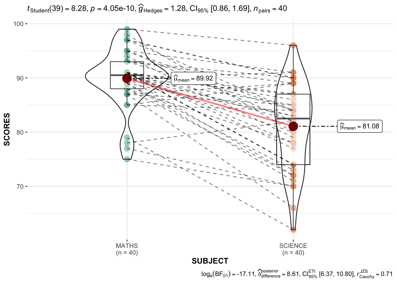
  filter(CLASS == "3A")

ggwithinstats (
  data = filter(exam_long, 
                SUBJECT %in%
                  c("MATHS", "SCIENCE")),
  x = SUBJECT,
  y = SCORES,
  type = "p"
)

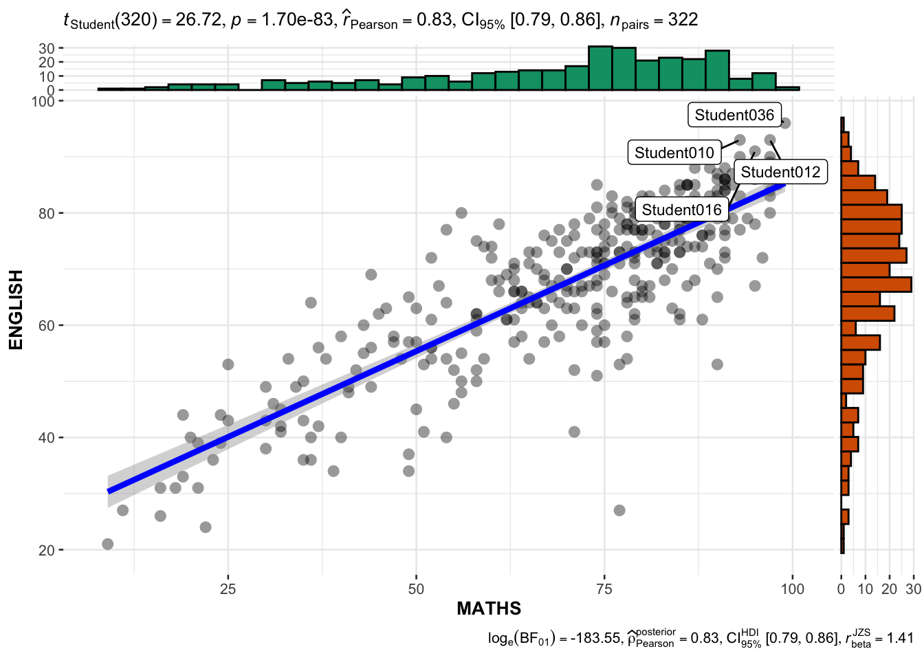
ggscatterstats(
  data = exam,
  x = MATHS,
  y = ENGLISH,
  marginal = TRUE,
  label.var = ID,
  label.expression = ENGLISH > 90 & MATHS > 90,
)

Toyota sales exercise

pacman::p_load(readxl, performance, parameters, see)

car_resale <- read_xls("data/ToyotaCorolla.xls", "data")
car_resale

# A tibble: 1,436 × 38
      Id Model    Price Age_08_04 Mfg_Month Mfg_Year     KM Quarterly_Tax Weight
   <dbl> <chr>    <dbl>     <dbl>     <dbl>    <dbl>  <dbl>         <dbl>  <dbl>
 1    81 TOYOTA … 18950        25         8     2002  20019           100   1180
 2     1 TOYOTA … 13500        23        10     2002  46986           210   1165
 3     2 TOYOTA … 13750        23        10     2002  72937           210   1165
 4     3  TOYOTA… 13950        24         9     2002  41711           210   1165
 5     4 TOYOTA … 14950        26         7     2002  48000           210   1165
 6     5 TOYOTA … 13750        30         3     2002  38500           210   1170
 7     6 TOYOTA … 12950        32         1     2002  61000           210   1170
 8     7  TOYOTA… 16900        27         6     2002  94612           210   1245
 9     8 TOYOTA … 18600        30         3     2002  75889           210   1245
10    44 TOYOTA … 16950        27         6     2002 110404           234   1255
# ℹ 1,426 more rows
# ℹ 29 more variables: Guarantee_Period <dbl>, HP_Bin <chr>, CC_bin <chr>,
#   Doors <dbl>, Gears <dbl>, Cylinders <dbl>, Fuel_Type <chr>, Color <chr>,
#   Met_Color <dbl>, Automatic <dbl>, Mfr_Guarantee <dbl>,
#   BOVAG_Guarantee <dbl>, ABS <dbl>, Airbag_1 <dbl>, Airbag_2 <dbl>,
#   Airco <dbl>, Automatic_airco <dbl>, Boardcomputer <dbl>, CD_Player <dbl>,
#   Central_Lock <dbl>, Powered_Windows <dbl>, Power_Steering <dbl>, …

Multiple Regressions using lm()

model <- lm(Price ~ Age_08_04 + Mfg_Year + KM + 
              Weight + Guarantee_Period, data = car_resale)
model

Call:
lm(formula = Price ~ Age_08_04 + Mfg_Year + KM + Weight + Guarantee_Period, 
    data = car_resale)

Coefficients:
     (Intercept)         Age_08_04          Mfg_Year                KM  
      -2.637e+06        -1.409e+01         1.315e+03        -2.323e-02  
          Weight  Guarantee_Period  
       1.903e+01         2.770e+01  

Checking and plotting multicollinearity

check_c <- check_collinearity(model)
plot(check_c)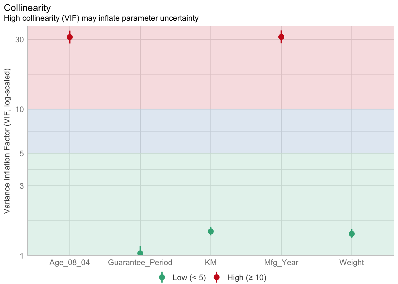

Checking for nomality assumption

model1 <- lm(Price ~ Age_08_04 + KM + 
              Weight + Guarantee_Period, data = car_resale)

check_n <- check_normality(model1)
plot(check_n)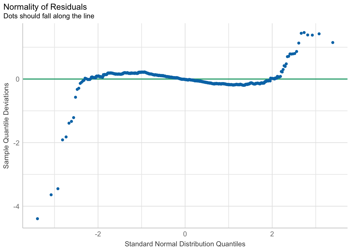

Model Diagnostic: Check model for homogeneity of variances

check_h <- check_heteroscedasticity(model1)
plot(check_h)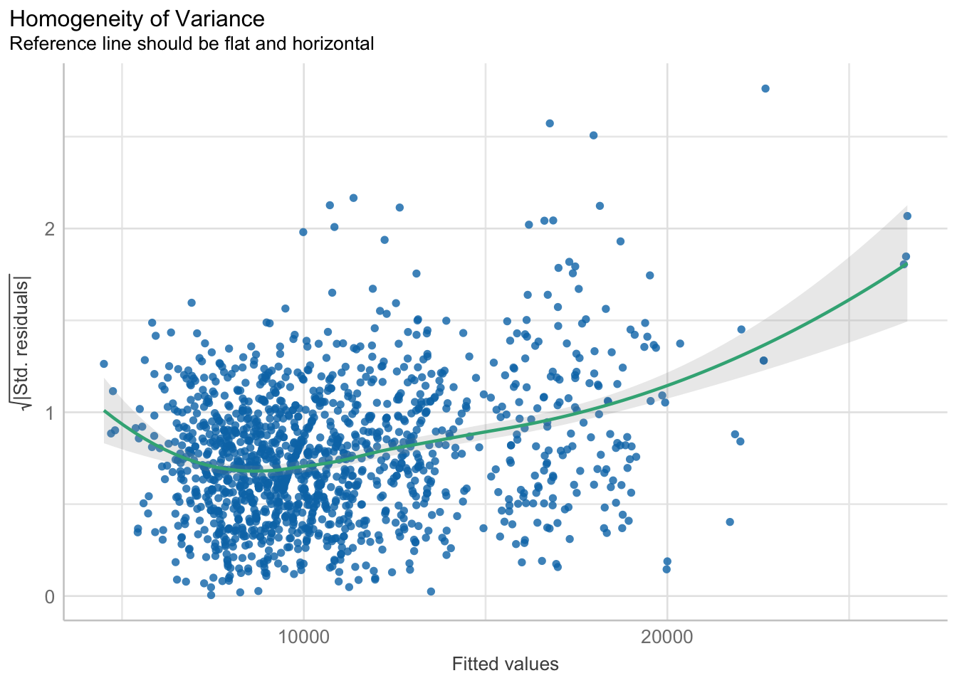

Model diagnostic: Complete check

check_model(model1)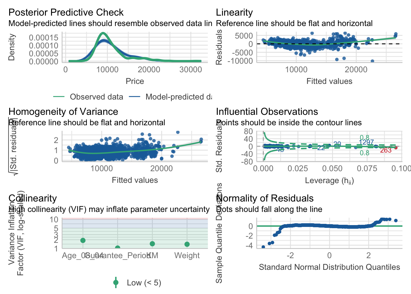

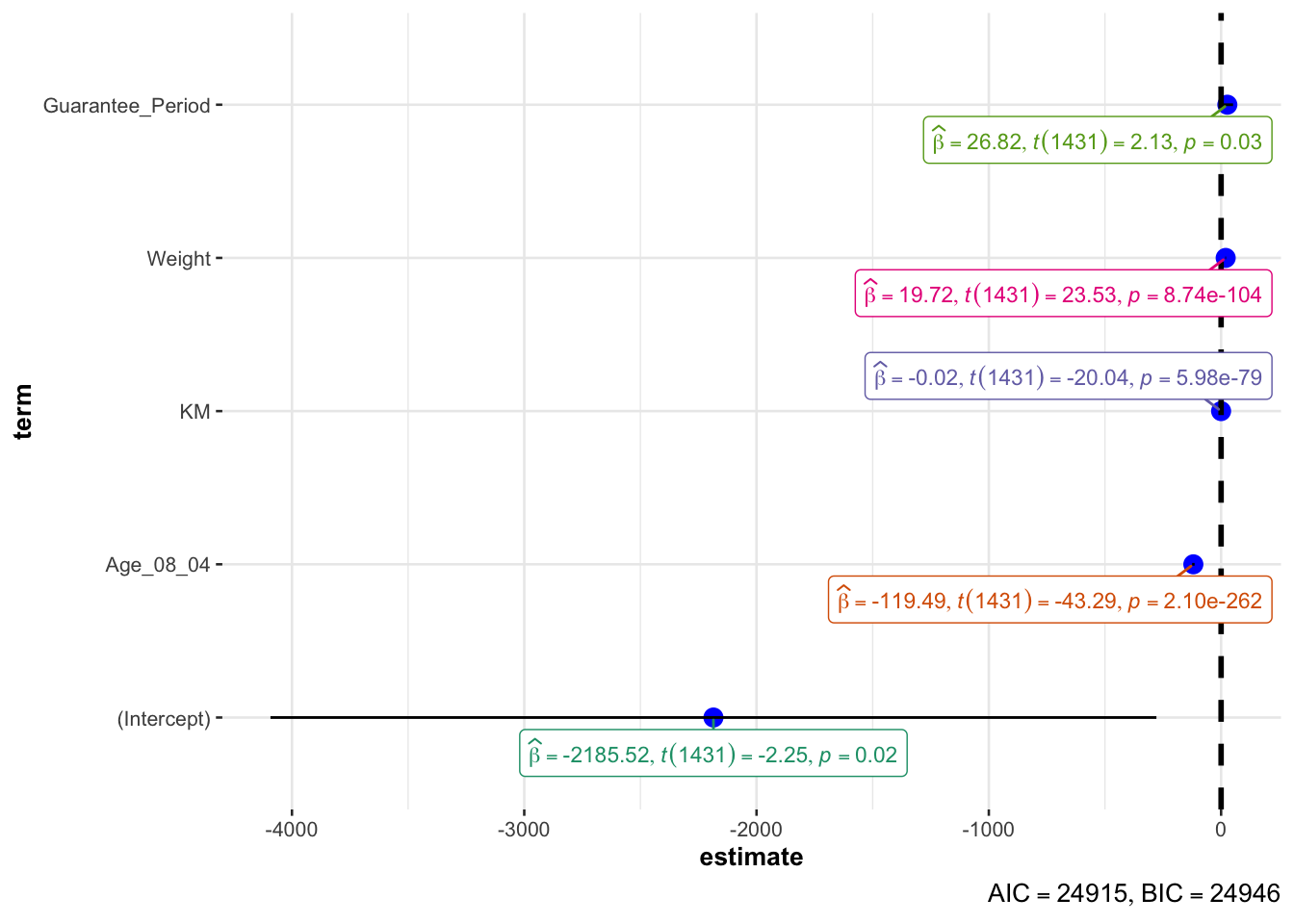
Visualising Regression param

plot(parameters(model1))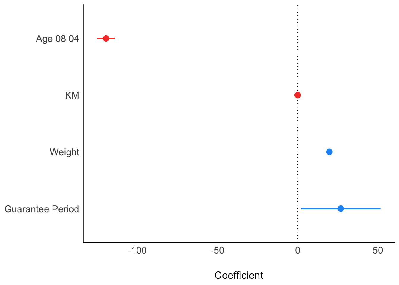

ggcoefstats(model1, 
            output = "plot")